Week 1: Introductions

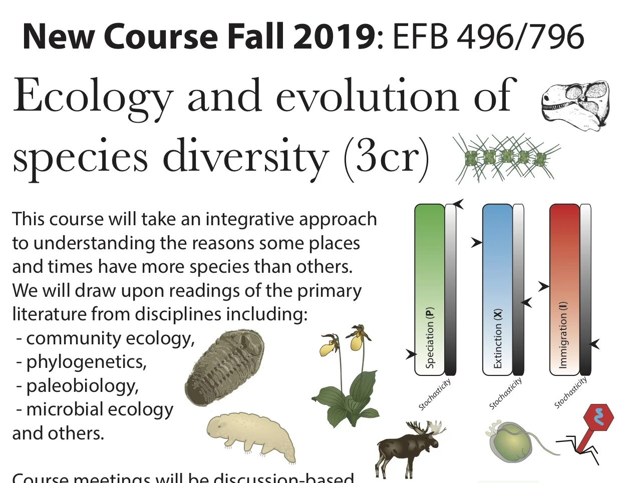
Today, we talked about the central question of this course: why are there more species in some places and times than in others? We very superficially acknowledged that “species diversity” can be tough to measure and assign biological meaning to, and then bustled along to talking about pattern and process. 

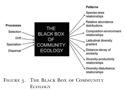
The number of species in a study system (a pattern we can observe) is the result of up to four processes:

• Speciation

• Selection

• Dispersal 

• Drift

Vellend 2010 (the source for the thumbnail pic) is a nice (and highly cited) synthesis that talks about how the importance of each process might be scale- and situation- dependent. Scale is a topic we’ll come back to repeatedly in this course. For a quick preview, see here and here.  

Vellend was certainly not the first to suggest that the number of species in an assemblage can be understood as the interplay among a limited number of processes, but previous authors generally codified it as Speciation, Dispersal, and Extinction (or, depending on the scale of the study, extirpation). Here, the paleontologist Fischer refers to these processes in the context of the latitudinal diversity gradient in a publication from 1960 

And below MacArthur & Wilson (1963) suggest the number of species on an island can be understood as the result of an equilibrium between immigration and extirpation (both were well aware of speciation, but did not incorporate it in their model). 

Vellend’s work is notable for separating out the extinction (or extirpation) term into a deterministic and stochastic component, just like selection and drift are treated in population genetics and microevolution. Ecological selection means a population abundance is going up or down due to repeatable interactions between its traits and environment (biotic and/or abiotic); whereas ecological drift is when the abundance of a population goes up or down randomly. Our meeting next week (week 2) is going to revolve around Vellend’s idea of ecological drift, and its analogy to genetic drift. (A brief note about replaying the tape of life: it’s an important part of our understanding of community assembly and evolution, and it’s sometimes definitionally tied to our understanding of drift and neutrality) We’ll also talk about neutral theory in ecology and its analogy to neutral theory in molecular evolution next week... So more on that, soon. 

Ricklefs 1987 is perhaps the most important intermediary synthetic publication between these mid-century synthetic treatments of species richness patterns and processes and Vellend 2010. Ricklefs 1987 is important in clarifying the importance of spatial scale and historical processes in understanding the structure of local communities. And in some places he closely foreshadows the way Vellend 2010 treats the contribution of “drift” to assemblage membership: "In simple laboratory systems, competitive exclusion requires on the order of 10 to 100 generations (47). Stochastic (chance) extinction depends on the size of the population, but if n is 1000 individuals (very small), an average extinction time of 10,000 generations is plausible (48). These periods seem brief compared to the production of species, changes in climate and positions of landforms, and appearances of new genotypes that enable populations to expand ecologically into new communities. However, migration of individuals between local systems with different equilibria may slow the rate at which interactions between species move a system to a local equilibrium, perhaps to a level approaching the scale of evolutionary and biogeographic processes." Please see the ongoing course glossary for additional notes on drift and stochastic extinction.

This line from the recent paper by Rapacciuolo & Blois sums up a lot of the central difficulties we’ll encounter throughout this course: “Even when reliable pattern–process connections have been made, seldom have they led to general ecological theories, due to the high contingency of those connections on the spatial, temporal and taxonomic scale of study (Simberloff 2004, Vellend 2010).” There’s a lot to unpack in this sentence. Pattern-process relationships are scale-contingent and history-contingent (this is a central part of Lawton’s 1999 lament), and “scale” can come in a number of flavors (spatial, temporal, taxonomic). People have been seeking order in community ecology for a long time. We’re likely to leave this class with more questions than answers.

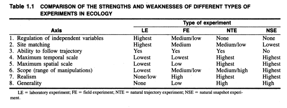
Speaking of questions and answers, we also talked a little bit about how we know what we know, unpacking Diamond’s classification of experiments. According to his very influential 1986 chapter, there are four main types of experiments ecologists participate in: 

• Lab experiments

• Field experiments

• Natural snapshot experiments

• Natural trajectory experiments

The whole chapter is worth a read, but I think the most important takeaway for our purposes is table 1.1, which you should keep in mind as you read papers for this course. What are the advantages and limitations of the methods the researchers used, based on their type of experiment? 

His chapter is particularly influential because it made it easier for ecologists to articulate the validity of natural experiments. There are some very profound questions that need to incorporate data from natural experiments, like understanding the latitudinal diversity gradient, or changes in regional diversity throughout the Phanerozoic (not to mention lots of questions in meteorology, geology, and cosmology). This is easy for biogeographers and paleobiologists to understand, but Diamond’s chapter might help you explain this to someone more used to doing experiments on a lab bench. 

There are definitely important advances to our understanding involving experiments that don’t neatly fit in these categories. Mesocosm and microcosm experiments are really important in aquatic and microbial ecology. These categories blend some of the benefits of laboratory and field experiments. And simulation studies have also substantially advanced our knowledge of diversity patterns and processes (e.g.: Raup et al. 1973; Pontarp et al. 2019). Finally, there are a variety of approaches to experimental evolution that are potentially relevant to understanding species diversity patterns.  

I put the other stuff we went over in a “Course resources” blog post, since you might want to come back to it. Be sure to check out that post, too! See ya Tuesday!